ETN-FPI TS2

Yes, it’s acronym time — by ETN-FPI TS2, I mean the second Training School of the European Training Network on Full-Parallax Imaging, which was held at the University of Valencia in September 2016. Chris Kaspiris-Rousellis and I attended, and had a marvellous time learning about optics. I had done some geometrical and wave optics as part of my undergraduate physics degree, but it was great to get back to it, refresh my memory and learn more. The course was brilliantly run by Manuel Martinez and Genaro Saavedra, and consisted of morning lectures followed by afternoon practical sessions in the laboratory.
img_7915
img_7963small
img_7947cropsmall
jroptics2
img_7972small

Mantis videos

In our lab, we run experiments on praying mantis vision. We show the insects videos on a computer (mainly boring stimuli like bars moving, or little black dots which are meant to simulate a bug) and video how they move, via a webcam. The webcam stores a short video clip for each trial. The webcam is positioned so it films only the mantis, not the computer screen. At the moment the experimenter then manually codes the video, making a simple judgment like “mantis looked left”, “mantis moved right”, “mantis did not move” etc.
Here are some example video clips of mantids responding to different visual stimuli.
We would love to be able to analyse these automatically, e.g. to get parameters such as “angle through which mantis head turns” or “number of strikes”.
As you can see, this is pretty challenging. There are big variations from experiment to experiment, and smaller variations from session to session even within the same experiment. The overall lighting, the position of the mantis, what else is in shot, etc etc, all vary.


Online lectures on the human visual system

I recently organised a Training School on 3D Displays and the Human Visual System as part of the European Training Network on Full-Parallax Imaging. The Network aims to train up 15 Early Stage Researchers who not only have expertise both in optics and engineering, but who also have an understanding of human visual perception. This first Training School aimed to equip the researchers, from a variety of disciplinary backgrounds but mainly engineering, with the relevant knowledge of the human visual system.

As part of this, I gave three lectures. I’m sharing the videos and slides here in case these lectures are useful more widely. Drop me a comment below to give me any feedback!

Lecture 1: The eye.


Basic anatomy / physiology of the eye. Photoreceptors, retina, pupil, , lens, cornea. Rods, cones, colour perception. Dynamic range, cone adaptation. Slides are here.

Lecture 2: The human contrast sensitivity function.


Disparity, stereopsis. Stereoacuity and stereoblindness. Binocular vision disorders: amblyopia, strabismus. The correspondence problem. Issues with mobile eyes; epipolar lines, search zones. Different forms of human stereopsis: fine/coarse, contour vs RDS. Slides are here.

Lecture 3: Stereopsis.


Spatial and temporal frequency. Difference between band-pass luminance CSF and low-pass chromatic CSF; applications to encoding of colour. Fourier spectra of images. Models of the CSF. Slides are here.

Brainzone

The Brain Zone advisory committee with Dame Eliza Manningham-Buller (in blue), the chair of the Wellcome Trust board of governors, at the launch of the new exhibition at the Centre for Life.

Dated: 13/04/2016 The Baroness Manningam-Buller – former head of MI5 and chair of Wellcome Fund – is visiting the Centre for Life in Newcastle Upon Tyne for the launch of the brain zone exhibition.  Fao Nicola McIntosh, Centre for Life.  #NorthNewsAndPictures/2daymedia

Dated: 13/04/2016
The Baroness Manningam-Buller – former head of MI5 and chair of Wellcome Fund – is visiting the Centre for Life in Newcastle Upon Tyne for the launch of the brain zone exhibition.
Fao Nicola McIntosh, Centre for Life.
#NorthNewsAndPictures/2daymedia

Eye tracking with small children using a touchscreen

Back in 2011, my then colleague Dr Catherine O’Hanlon and I carried out a study in which young children gave responses using a touchscreen, while we simultaneously tracked their eye movements. I’ve been asked a few times by other researchers about how we managed this, so I thought it would be useful to share some information here.
Setup

Here (8Mb) you should be able to download a Powerpoint presentation I gave to EyeTrackBehavior in 2011. It’s about the practical issues rather than the science, with photos of our set-up and videos of the experiments.

Some code fragments for using the SMI RED eye tracker with Matlab are here.

I’ve also uploaded a zip file (62Mb, compressed with 7-zip) containing the complete Matlab code, audio clips and images we used to run our experiments. This worked in 2011 but no longer runs on my version of Matlab in 2016 so don’t expect it to work for you. However, it might possibly be useful for anyone aiming to do something similar so I thought why not share it.

Outreach: maths week at Shotton Hall Academy

This week I had an opportunity to speak to some aspiring mathematicians about their future and to ask them to think about maths. Not just to answer the questions, and not to just ask ‘why’ without purpose, but to try and find a middle ground between the two. I also obviously tried to include some of the research the institute does, to tie it to my own research.

The first thing I asked the kids to do was to explain to me an example of using maths. Most of them came up with some interesting ideas that focused on measuring quantities and making calculations. I then asked them to come up with a definition. They all said similar things, all along the lines of ‘measuring, calculating, and using data’. Which is a great answer! But was not what I was looking for. ‘OK, give me an example of something that doesn’t use maths.” was my next question. A few hazarded some guesses and were all shown that maths IS in there somewhere! We agreed that a great definition of maths would be that it is simply problem solving. Everything else you do with maths is simply a tool to solve the problem with.

I then talked about earnings and aspirations of mathematicians (did you know that aside from medicine the maths degree is the best paid degree to have in the world?) and went into my own mathematical work. Not the modelling (bit too complicated for 15 year olds) but the actual calculations of the parallax. We went through an example and the kids had to answer the question themselves. They had to solve the problem, I didn’t spoon feed it to them. I think this made for interesting discussion.

That was the end of it, just time to wrap up (DO MATHS AT A LEVEL) and then to give them all a brain sweet for taking part so nicely. All in all I think it went well!

Percentage of variance explained

I was just looking for a good explanation of this online to point a lab member towards, and I couldn’t find anything suitable, so I thought I’d write something myself. (Since then, this https://en.wikipedia.org/wiki/Fraction_of_variance_unexplained seems pretty good.

The idea is you have a set of experimental data {Yi} (i=1 to N). These might be responses collected in N different conditions, for example.
The mean is

M = sum{Yi} / N

and the variance about this mean is the total variance

TV = var(Yi) = sum{ (Yi-M)^2 } / N

Now suppose you have some model or fit which predicts values Fi. The residuals between the fit and the data are Ri=(Yi-Fi). The mean of the squared residuals is

RV = sum { (Yi - Fi )^2 } / N

(this is identical to the variance of the residuals if Fi and Yi have the same mean, as they do in linear regression)
The fraction of UNexplained variance is RV/TV, so the fraction of explained variance is 1-RV/TV.

In a perfect world, Fi would be equal to Yi for all i, and therefore these residuals would all be zero. RV=0 and thus all of the variance is explained. The other end of the spectrum is where all the fit values are the same, just equal to the mean of the data: Fi=M. Then we can see from the equations above that RV=TV and none of the variance is explained.

The percentage of variance which is explained is

PV = 100(1-RV/TV).

On Converting Pixels to Degrees

The Warping Effect

In our mantis contrast sensitivity paper (http://tinyurl.com/mantiscsf) we used the following formula to calculate the spatial frequency of grating stimuli in cycles per degree (cpd):

eqn

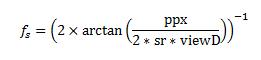
Where ppx is the grating period in pixels, sr is the screen resolution in px/cm and viewD is the viewing distance in cm.

This equation assumes a linear correspondence between screen pixels and the visual angle subtended by these pixels (in degrees). The conversion ratio is effectively the average over one grating period; for example a spatial period of 100px corresponds to 20.25 degs making the effective conversion ratio 4.94 px/deg.

When viewD is sufficiently large (which is typical for human experiments) the assumption of a linear correspondence between screen pixels and angle subtended holds (i.e. differences are negligible). However, for small viewD there could be considerable differences as gratings subtend smaller angles the further they are from the centre and thus the stimulus appears to be “squeezed” near the screen ends.

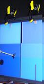
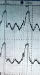
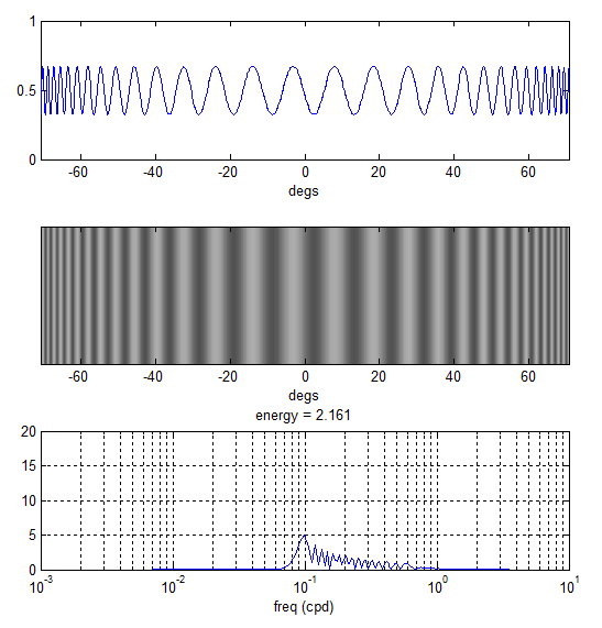
The plots below demonstrate this effect. The top two plots show a horizontal sinusoidal grating of period 5 px (sr = 40 px/cm) as perceived by an observer 7cm away from the monitor. Instead of a constant frequency in cpd there is actually a range of frequencies going from low (at the screen centre) to high (at both ends). The bottom plot is a frequency spectrum showing how broadband this actually is. Using the equation above fs = 0.978 cpd for this stimulus while the actual spectrum goes from 0.08 all the way up 0.6 cpd.

spec1

How to correct for this

One way to correct for this is to incrementally increase the grating period as we move away from the screen centre. For an observer standing sufficiently away from the monitor such a stimulus would appear squeezed at the centre and stretched at the sides. At the right viewing distance, however, all gratings will subtend the same visual angle.

This can be done in multiple ways in Matlab. I’ve found the following particularly intuitive and easy to implement:

  1. Calculate the visual degree corresponding to each px on the screen given a viewing distance and a screen resolution (the function px2deg does this for you)
  2. Use the obtained degrees array to calculate grating/stimuli luminance level

For example, to render a sinusoidal grating of frequency 0.1 cpd on a monitor that is 1920px wide I do:

scrWidthPx = 1920; % px
screenReso = 40; % px/cm
viewD = 7; % cm
freq = 0.1; % cpd
degs = px2deg(scrWidthPx, screenReso, viewD);
y = cos(2*pi*degs*freq);

The array y now contains 1920 luminance levels which, when rendered horizontally across the 1920 screen pixels, would simulate a grating of 0.1 cpd at the specified viewing distance. The plots below demonstrate how this is perceived by the observer.

spec2

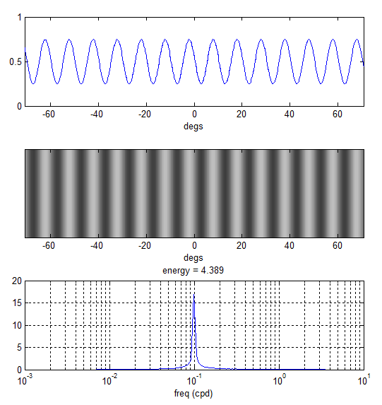
The rendered stimulus is now narrow-band as intended.

 Precautions

The correction above assumes a certain viewing distance and that the observer is positioned laterally in front of the screen centre. If the observer position changes then the perceived stimulus will have a different spectrum and so it is important to ensure that subjects (in our experiments, mantids) are placed at the correct viewing distance both away from the screen and laterally to minimize any errors.

How does this affect our CSF Data

The “warping effect” that we described above must be taken into consideration when interpreting the data we published in the mantis CSF paper. Each spatial frequency we rendered was actually perceived by the mantis as a broadband signal and so the actual mantis CSF is likely more narrow-band compared to what we reported.

Which Windows/Matlab version with Psychophysics Toolbox?

My colleague Nicholas Port was just asking me about my experience with different versions of Windows & Matlab running Psychophysics Toolbox. I asked my team about their experience, and I thought it might be useful to record their comments here:

Paul: “I used windows 7 and Matlab 2012b for psychophysical experiments before and I didn’t have any issues. However when I was using an Eyelink 1000 (external eyetracker) and timing was important for some reason the functionality only worked on 64 bit, so it is certainly worth considering which version you should use. Windows 7 and 2012A is more than enough.”

Zoltan: “I used Windows 8.1 with Matlab R2014A. I had some issues with timing because the desktop mode is handled differently.
If you do production-quality stuff where timing is important, go with Windows 7 for the time being. I never had any issues with the 64-bit Matlab. However, there is a software limitation with Windows 7: the refresh rate you can set on any monitor is capped at 85 Hz. You will need to do some hacking in the registry if you have a Radeon card, and you can conveniently make a new custom resolution with anything nvidia.
So, currently, the most stable stuff is a Windows 7 PC, 64-bit Matlab, and an nVidia GPU. If you need more power, switch off the swap file, visual effects and have plenty of RAM.”

Ghaith: “I’ve been using PTB on Windows 7 using both 32/64-bit versions of Matlab with no problems.”

Partow: “I had some problems in downloading psychtoolbox with 32-bit on a Windows 7. 64 is fine.”