


This is code developed for and described in the paper “What-Where-When memory is unimpaired in healthy people over 70” by Mazurek, Bhoopathy, Read, Gallagher, Smulders.
The code enables you to compute the Bayes Factor to assess whether two groups (in our paper: Younger and Older people), differ in their performance on a binomial task. By binomial task, we mean one consisting of N discrete trials each with two outcomes (in our paper: correct or incorrect).
Members of the Young group performed NY trials and were correct on a total of MY, a performance level of MY/NY.
Members of the Old group performed NO trials and were correct on a total of MO, a performance level of MO/NO.
The null hypothesis is that the probability of being correct on any given trial is the same for all participants, in both groups. The experimental hypothesis is that the probability is different in the two groups (but the same for all members of a given group, on all trials).
The Bayes Factor computes the likelihood of the observed difference in performance under the experimental hypothesis, divided by the likelihood under the null hypothesis.
You can run this code as a Matlab GUI by downloading the following files:
BayesFactor.m
BayesFactor.fig
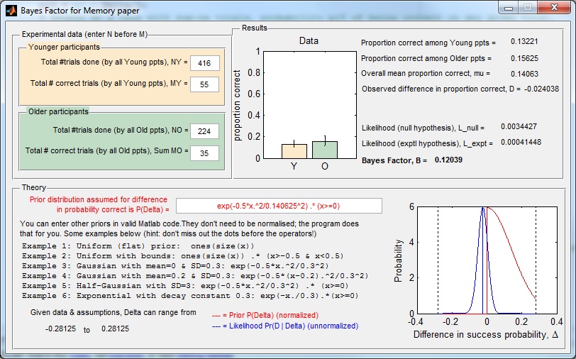
Just copy them to a folder, navigate to this folder in Matlab and type “BayesFactor” in the command window. You should see a GUI like this:
A Russian correspondent tells me that the download doesn’t work if you enter your name in non-Latin characters — sorry about that; please use the Latin alphabet as a work-around.
If you do not have Matlab, you should be able to download an installer here which will enable you to run the program on Windows.
.
Email me if that doesn’t work!
Documentation
The GUI fires up with the values for one of the experiments in our paper. You can enter new values. It won’t let you enter negative values, or 0 for the total number of trials. It also won’t let you enter a number of correct trials which is greater than the total number of trials, so make sure you change the total before you change the number correct.
The bar chart in the “Results” panel shows the proportion correct for the two groups, based on the numbers you have entered in the “Experimental data” panel. The error bars show 95% confidence intervals based on simple binomial statistics (Agresti, A. and Coull, B. A. (1998). Approximate is better than “exact” for interval estimation of binomial proportions, The American Statistician, 52(2), 119-12).
In the “Theory” panel, you can alter the prior for the difference Delta in the probability of being correct, between age-groups. Positive values of Delta mean that young people perform better than older people. We used a half-Gaussian – so yes, we ruled out a priori the idea that old people could possibly do better than young people. You may have your own prior, in which case feel free to enter it by typing in the text box with red writing. You can enter any function you want, in valid Matlab syntax. Some examples are given below. When you press return, the new prior function will be drawn in red on the axes on the right. As it says, the program automatically normalises this so you don’t have to worry about that.
The blue curve shows the likelihood of the data, i.e. the probability of getting the observed difference D in the proportion correct, given the totals NY, NO you entered above, assuming that the true difference between groups in the probability of being correct is Delta. This is plotted as a function of Delta. The vertical blue line shows the observed difference in proportion correct. The likelihood distribution is not normalised, as otherwise it often would not be visible on the plot. The posterior distribution would be given by multiplying the red and blue curves together. The Bayes Factor is the area under this product curve, divided by the y-intercept of the blue curve.