Notes on using the DATAPixx with Psychophysics Toolbox, 2010

I recently bought a DATAPixx system from VPixx Technologies. It can do lots of things, but my motivation for buying it was (a) it allows 16-bit control of contrast (i.e. gray-levels from 0 to 65535, not the usual 0-255), with no restriction on what gray-levels you can use in a single frame, and (b) it can be used with a rather whizzy response box, RESPONSEPixx, which does micro-second accurate timing and has four buttons which you can light up to give cues to subjects. Here are my notes on using the system. Many thanks to Peter April and Jean-Francois Hamelin at VPixx who provided fabulous technical support throughout.

My set-up

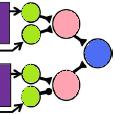
Here’s how I had the DATAPixx system connected for my original experiments.

I subsequently moved to running in Linux. I was using a dual-head NVidia GeForce G210 graphics card, and my monitors are two Compaq CRTs, a P1210 and P1100. Both are capable of 160Hz at 800×600. See my notes on high refresh rates. Later on I moved to high frame rates under Windows.

Drivers

To use the DATAPixx with Windows, you need to install the drivers. It comes with instructions how to do this. Initially I was using the DATAPixx with Windows 7; VPixx sent me a special driver for use with this OS. Right now I’m using the DATAPixx with a Linux machine; you don’t appear to need any special drivers for this. However, as I discovered, you do need the freeglut package installed.

Some old code

Ignore this; it’s now been superseded by improvements to Psychtoolbox. Psychtoolbox now makes it really easy and fast to display stimuli on the DATAPixx. But I left this up just in case I ever want to refer to it.

DATAPixx has three video modes. I have been using Video Mode 2. The second argument of DATAPixx_ConvertImage.m specifies which mode you want:

• 0 = no DATAPixx, just scale the 16-bit image down to 8-bits, i.e. losing contrast resolution;
• 2 = DATAPixx video mode 2. In this, the high 8 bits of your image go into the red channel, and the low 8 bits go into the green channel. This enables an 8-bit graphics card to send a 16-bit monochrome image, using your full screen.
• 3 = DATAPixx video mode 3. In Peter April’s words, “Video Mode 3 implements 16-bit RGB resolution by taking 2 adjacent 8-bit RGB input pixels to generate 1 16-bit RGB output pixel.  This necessarily halves the horizontal resolution.  For example, if your display is configured for 1024×768 8-bit pixels, then your original PsychToolbox image which you are converting should really be 512×768.  If you want to have a final resolution of 1024×768 16-bit RGB pixels, then you can configure your display to be 2048×768 using a utility like PowerStrip from http://www.entechtaiwan.com/util/ps.shtm .” This is what you would do if you wanted to display 16-bit colour images on your DATAPixx, but I have no need to do this at present, and thus video mode 2 does me fine.

I originally started using the DATAPixx just opening a PTB window with Screen(‘OpenWindow’), manually writing my image as a matrix suitable to be sent to the DATAPixx. To do this, I wrote DATAPixx_ConvertImage.m. This is a Matlab file which takes a 16-bit stimulus matrix (i.e. an array of numbers between 0 and 65535), and outputs a matrix suitable for passing to the DATAPixx.

In my Matlab code, then, I can write:

% Define parameters:
maxpixval = 2^16-1;
datapixxmode = 2;
stimulusmonitor = 1;
[screenx, screeny ] = Screen(‘WindowSize’,stimulusmonitor);
% Prepare DATAPixx:
Datapixx(‘Open’);
Datapixx(‘SetVideoMode’,datapixxmode);
Datapixx(‘StopAllSchedules’);
Datapixx(‘RegWrRd’);
% Make stimulus:
noise = rand(screeny,screenx )*maxpixval ;
noise = DATAPixx_ConvertImage(noise,datapixxmode );
% Display stimulus:
window = Screen(‘OpenWindow’,stimulusmonitor );
noisetex=Screen(‘MakeTexture’, window, noise );
Screen(‘DrawTexture’,window,noisetex);
Screen(‘Flip’,window);

That should display 16-bit noise on your screen.

 

Using the DATAPixx with Psychophysics Toolbox

Thanks to Mario Kleiner and Peter April, it’s now really easy and fast to use the DATAPixx box via the Psychtoolbox imaging pipeline. There’s a Datapixx toolbox with special commands to interface with the DATAPixx, but in fact you may not even need to use that. There are now special Psychimaging commands e.g. “EnableDataPixxM16Output”, to quickly get 16-bit monochrome output, or “EnableDataPixxC48Output” for 16-bit colour, without the user needing to worry about the details of how to get that information to the DATAPixx. You simply define your image as a matrix from 0 (black) to 1 (white), and store it with 32-bit precision. NB this is a bit different from the usual PTB language where 255=white. The point is that it enables you to smoothly move between different numbers of bits, using the same code.

One-time system set-up

Before using the DATAPixx for the first time (including after changing screen resolution etc), run two set-up codes which get everything sorted out, iron out any problems with the LUTs, etc.

BitsPlusImagingPipelineTest(screenID);
BitsPlusIdentityClutTest(screenID,1); % where 1 means “use the DATAPixx”

and answer “y” to questions about use DATAPixx diagnostics. That done, you can start displaying stimuli.

Displaying stimuli using PsychImaging

To see how this works, here is some code Peter April supplied me with.

To get everything up and ready to go, and open a PTB window for display on monitor screenNumber:

AssertOpenGL;
% Configure PsychToolbox imaging pipeline to use 32-bit floating point numbers.
% Our pipeline will also implement an inverse gamma mapping to correct for display gamma.
PsychImaging(‘PrepareConfiguration’);
PsychImaging(‘AddTask’, ‘General’, ‘FloatingPoint32Bit’);
PsychImaging(‘AddTask’, ‘General’, ‘EnableDataPixxM16Output’);
PsychImaging(‘AddTask’, ‘FinalFormatting’, ‘DisplayColorCorrection’, ‘SimpleGamma’);
oldVerbosity = Screen(‘Preference’, ‘Verbosity’, 1); % Don’t log the GL stuff
[win, winRect] = PsychImaging(‘OpenWindow’, screenNumber);
Screen(‘Preference’, ‘Verbosity’, oldVerbosity);

Now, you define your image as a matrix from 0 (black) to 1 (white), storing it with 32-bit precision. You then display it with DrawTexture. Here’s an example from Peter:

% define a 2D plaid with 100% contrast and 256 pixel period, with value in the range 0-1.
[wx,wy] = meshgrid(1:winWidth, 1:winHeight);
plaidMatrix = (sin(wx*pi/128) + sin(wy*pi/128)) / 4 + 0.5;
% Make a 32-bit floating point monochrome texture out of it.
% The “2” entry says using floating precision. plaidTexture = Screen(‘MakeTexture’, win, plaidMatrix, [], [], 2);
% Draw the floating point texture.
% Specify filter mode = 0 (nearest neighbour), so that GL doesn’t interpolate pixel values.
Screen(‘DrawTexture’, win, plaidTexture, [], [], [], 0);
Screen(‘Flip’,win);

Or, you can use the usual Psychtoolbox commands, like FillRect and so on, just defining your colours between 0 and 1 not 0 and 255. I haven’t yet encountered any problems with this; it all seems to work as expected.

Things to note

Do not use LoadNormalizedGammaTable with the DATAPixx. I originally had a line

% Ensure that the graphics board’s gamma table does not transform our pixels
Screen(‘LoadNormalizedGammaTable’, w, linspace(0, 1, 256)’ * [1, 1, 1]);

but Mario Kleiner gave me the following dire warning: “Not needed, possibly harmful: The PsychImaging() setup code already calls LoadIdentityClut() which loads a proper gamma table. Depending on operating system and gpu the tables need to differ a bit to compensate for driver bugs. The LoadIdentityClut routine knows a couple of different tables for different buggy systems. The automatic test code in BitsPlusIdentityClutTest and BitsPlusImagingPipelinetest also loads an identity lut via LoadIdentityClut and tests if that lut is working correctly for your gpu – and tries to auto-fix that lut via an automatic optimization procedure if it isn’t correct. With your ‘LoadNormalized…’ command you are overwriting that optimal and tested lut, so you could add distortions to the video signal that is sent to the datapixx. A wrong lut could even erroneously trigger display dithering and add random imperceptible noise to the displayed image – at least that is what i observed on my MacBookPro with ati graphics under os/x 10.4.11.” (posted on Psychtoolbox forum, 3/9/2010)

Mario also advises adding the line

Options “FlatPanelProperties” “”Scaling = default, Dithering = disabled”

to either the Screen or Device section of your xorg.conf in /etc/X11 as described here. This ensures that the graphics card doesn’t try and do anything fancy dithering in the errroneous belief that your DATAPixx is a flatscreen monitor and that this will improve the appearance of colours. What it could actually do instead is introduce 1/256 luminance noise.

Also, you do not need to specifiy Screen(‘ColorRange’, w, 1, 0). According to Mario, this doesn’t hurt but is redundant as it is done automatically in high precision display mode.

 

Closing DATAPixx

To close everything down again afterwards, so you can run again without errors, just use “sca”. This closes the DATAPixx, restores the LUTs etc. I have found that the DATAPixx is not happy if my code crashes out with an error (which obviously happens all the time during development). The next time I run the code, it complains that DATAPixx cannot be opened (“check it is turned on and not in use with another program”). I haven’t found a way of recovering from this; I try Datapixx(‘Close’) and Datapixx(‘Reset’), but still get the same errors. Fortunately it’s simple to avoid; just make sure you put a catch in, like:

try
your code here
catch
lasterr
Priority(0);
clear all
sca
ShowCursor;
end

Which is good practice anyway when developing Psychtoolbox code.

Gamma correction with the imaging pipeline

Click here for some background on gamma correction. Peter April: “When using the DATAPixx, the pixel values which you program are the exact ones which are sent to the video DACs.  There is no further gamma table lookup. Note that this is the same as doing

Screen(‘LoadNormalizedGammaTable’,w,linspace(0,( 65535 / 65536), 65536)’*ones(1,3));

So, if you are using an LCD or similar display where in my experience (see here and here) there can be odd and unpredictable non-linearities between pixel value and luminance, you will need to transform your image appropriately before sending it to the DATAPixx.

If you are using a CRT, as I am for this experiment, and as you probably want to do if you are interested in fine contrast control, then luminance should be a power-function of pixel-value. Then, Mario Kleiner’s imaging pipeline has a function which can do this for the DATAPixx, and Peter April has given me demo code for this. NB Before using any PsychToolbox imaging pipeline routines, you have to do a 1-time system setup as described above.

Now, after opening the window using PsychImaging (not Screen), you can specify the window’s inverse gamma value to be applied in the imaging pipeline:

gamma = 2.2;
PsychColorCorrection(‘SetEncodingGamma’, win, 1/gamma);

NB As per Mario’s warning above, do not write to the LUT via Screen(‘LoadNormalizedGamma’)

Results of gamma-correcting a CRT using the DATAPixx and PsychImaging

I wrote DatapixxGammaCorrection.m to do gamma correction on a CRT. The monitor was a Compaq P1210 running at 160Hz, measured with a Minolta LS-110 photometer. As you can see in the figure below, it has worked extremely well. CRTs are such a joy compared with digital displays! The plot on the left shows luminance values recorded with gamma=1; this was fitted with a power-law to yield gamma=2.268. This was then used in

PsychColorCorrection(‘SetEncodingGamma’, win, 1/2.268);

and the luminance was measured again, resulting in the beautifully linear plot on the right.

Contrast control

The main reason I wanted the DATAPixx in the first place was to get fine control of contrast. I’d like to test this, but my photometer lacks the resolution to track 60 thousand-odd luminance levels! I wrote DatapixxExamineFineControl.m to have a look. This does 50 luminance measurements of each of 5 different pixel values: the gray level 32768 plus values 1, 2, 3,4 ,5 10, 20, 50 and 100 away from this.

Difference in pix-val	Pixel value (black=0, white=65,535)	Normalised pixel value (black=0, white=1)	Mean measured luminance (cd/m^2)	SEM of 30 repeats (cd/m2)
0	32768	0.500007629510948	46.307000000000002	0.014
1	32769	0.500022888532845	46.299666666666667	0.015
2	32770	0.500038147554742	46.312000000000005	0.014
3	32771	0.500053406576638	46.307666666666670	0.013
4	32772	0.500068665598535	46.308999999999997	0.013
5	32773	0.500083924620432	46.308000000000000	0.015
10	32778	0.500160219729915	46.322333333333326	0.017
20	32788	0.500312809948882	46.330333333333336	0.016
50	32818	0.500770580605783	46.381333333333330	0.014
100	32868	0.501533531700618	46.435999999999993	0.013

These values are shown in the following graph:

Clearly there is a lot of random noise, which I suspect is due to the photometer rather than the display. Equally obviously the photometer readings are quantised, and the steps between the luminance levels which the photometer can report are larger than the luminance difference expected for a 1-bit change in pixel value. Unsurprisingly perhaps, there is little visible consequence of pixel values differing by up to 5 (out of 2^16 possible values). However, there is a clear difference even at a difference of just 10. That is, on a scale where 0=black and 1=white, I can measure a difference in luminance between a gray-level of 0.5000 and one of 0.5002. I am pretty chuffed with this.

I also looked at a small number of pixel-values, doing 200 automated measurements of each one:

Difference in pix-val	Pixel value (black=0, white=65,535)	Normalised pixel value (black=0, white=1)	Mean measured luminance (cd/m2)	SEM of 200 repeats (cd/m2)
0	32768	0.500007629510948	46.195299999999968	0.0003857
1	32769	0.500022888532845	46.198199999999972	0.000391
2	32770	0.500038147554742	46.198399999999957	0.000387
3	32771	0.500053406576638	46.202199999999948	0.000383
4	32772	0.500068665598535	46.200999999999979	0.000383
5	32773	0.500083924620432	46.206799999999951	0.000392

Results shown below. I am actually pretty happy with this as it looks as if I can pick up the luminance difference caused by a change of just 2 out of 65,535:

That is, if I average over enough photometer measurements, I can detect the difference between 0.50000 and 0.50002. This confirms that I am indeed getting 16-bit contrast control from the DATAPixx. It is not an exhaustive test because of the noise on (I assume) the photometer, and because I was only testing whole-field stimuli.

I have also tested the 16-bit resolution with my own visual system. At low luminance levels, I can readily detect sine-gratings of very low amplitude. E.g., the Compaq P1210 CRT has a maximum luminance of 94.19 cd/m^2 and a min of 0.068 cd/m^2 according to my photometer, measured in the dark. I find that if I set the background luminance to a normalised pixel-value of 0.5, then I can only detect sine gratings with an amplitude of about 1/256 anyway, which I could display even without the DATAPixx. But if I set the background luminance to a pixel-value of 10/2^16, so that the same luminance step represents a much higher contrast, then I can readily detect a sine grating with an amplitude of 1/2^16. This must be due to my DATAPixx, as such a grating would be impossible to display with just 256 gray-levels — even with rounding, the peaks of the sine grating do not get up to even 1/256. So, I am pretty convinced the DATAPixx is acting as it should. Feel free to suggest any further tests I should do.

A note on Procedural Gabors

While using the DATAPixx at high refresh rates, I’ve found it incredibly useful to use Psychtoolbox’s Procedural Gabors. This is a brilliant way of doing drifting or flickering Gabors – it’s really fast, you only need to create one texture and then you can change its phase, and even orientation and frequency etc, on the fly. Like a much better version of the old LUT animation technique. And, it also works with 16-bit resolution. However, I found the parameters a bit hard to get my head around. If you are a vision scientist using Procedural Gabors to display visual stimuli, you almost certainly want to set disablenorm=1. The default value is 0, in which case the Gabor is normalised — then for a given value of the “contrast” input parameter, the Gabor’s peak amplitude depends on its spatial extent, which vision scientists typically don’t want. Here’s a code fragment:

disablenorm=1; % don’t do the normalisation
contrastpremult=0.5; % % Build a procedural gabor texture for a gabor with a support of tw x th pixels, and a RGB color offset of BGlum, the background luminance.
gabortex = CreateProceduralGabor(win, tw, th, nonsymmetric, [BGlum BGlum BGlum 0.0],disablenorm,contrastpremult);
…
% Then to actually draw a Gabor, do: Screen(‘DrawTexture’, win, gabortex, [], [], tilt, [], [], [], [], kPsychDontDoRotation, [phase freq sc con, aspectratio, 0, 0, 0]);

The Gabor parameters you pass to DrawTexture are mostly fairly standard, although I haven’t quite figured out where the zeros are:

• phase = phase in degrees.
• freq = carrier spatial frequency in cycles per pixel.
• sc = standard deviation of (here isotropic) Gaussian envelope, in pixels

The exception is the parameter I’ve called “con” above. Although this is described as “contrast” in the PTB documentation, it is not really contrast as vision scientists usually use the term, but (if I’ve understood correctly) amplitude. If disablenorm=1, then the amplitude of the Gabor will be

amp = contrastpremult * con

i.e. the carrier of the Gabor goes from mn=(BGlum-amp) to mx=(BGlum+amp), so its Michelson contrast is

Michelson contrast = (mx-mn)/(mx+mn) = amp / BGlum = con * contrastpremult / BGlum

So, if BGlum=0.5 (mid-grey background, which is usually what you want) and contrastpremult=0.5, then the parameter con = Michelson contrast. But in general, it won’t be. So be aware of that.

RESPONSEPixx

I like the RESPONSEPixx a lot. Unlike the Cedrus (in my hands anyway), it seems to be totally reliable — never misses a press. I like the ability to use the light-up buttons to cue subjects as to when a response is required, and which buttons are valid responses. It has a nice chunky feel, and will I think be much easier for patients than a mouse. It would have been very handy when I was testing the visually-agnosic Patient DF.

I had not realised in advance that it offers another advantage when presenting demanding stimuli. Normally, if I want to allow participants to respond during a stimulus, I have to poll the mouse or keyboard during stimulus presentation, which takes CPU time and risks dropped frames. With the DATAPixx system, the PC can just concentrate on presenting the stimulus, while the RESPONSEPixx logs any button-presses. At stimulus offset, the PC can then ask whether any buttons were pressed (and collect their exact times as well).

RESPONSEPixx_GetLastButtonPressed.m is a piece of code I wrote to help with this. It reads all button-presses currently in RESPONSEPixx buffer (since last flush or read). It ignores button releases, and just returns the identity of the last button pressed. If no button has been pressed, this returns an empty variable. Calling this function wipes the buffer, so if you call it twice in a row, the second time will be empty. The optional second argument gives the time at which the button-press was made, in seconds since the Datapixx was powered up. If you want this in seconds since stimulus onset, for example, then you need to do something like

Datapixx(‘RegWrRd’);t0=Datapixx(‘GetTime’);
(stimulus generation code)
[button,t1] = RESPONSEPixx_GetLastButtonPressed;
reactiontime = t1-t0;