


Thanks to Damon Clark at Yale and Jacob A. Zavatone-Veth at Harvard for pointing out the following to me.
I had always thought that you could get a direction-selective neuron with a linear filter that is spatiotemporally inseparable, so that it is “tilted” in spacetime, with the gradient defining a speed and direction. I always thought you would get a bigger response for a stimulus moving at the speed and in the direction matching the filter, than for one moving in the opposite direction. I know models, like the motion energy model, then tend to place a nonlinearity after the linear filtering, but I didn’t think this was necessary for direction-tuning when the filter is already tilted in this way.
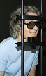
Well… yes it is (although it does slightly depend on what you mean by direction-selective). The video below shows a Gaussian-blob stimulus passing over a receptive field, first left to right and then right to left.
The leftmost panel shows the tilted spatiotemporal linear filter representing the receptive field. How to read this function: It responds weakly to the present stimulus (tau=0), responding most to stimulation at x=-50. It responds more strongly to stimuli as we go back into the past. It responds most strongly to stimuli that were presented at a time tau=40 units ago, located at x=-11. As we go further back into the past, its responds decays away. It responds weakly to stimuli presented 70 time-units ago, most strongly to those that were at x=10 units 70 time-units ago. This panel doesn’t change, as the filter’s shape is a permanent feature (it’s time-invariant).
The middle panel shows the stimulus. The bottom row (tau=0) shows where the stimulus is now; the rows above show where it was at times progressively further into the past. At any given moment of time, the stimulus is a Gaussian function of position. The contour lines show the filter for comparison.
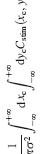
The right-hand panel shows the response of the linear filter, which is the inner product of the filter and the stimulus at every moment in time.
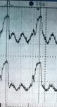
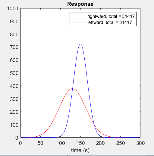
The red curve shows the response when the stimulus moves rightward; the blue curve shows the response when the stimulus moves leftward.
Here is the response as a function of time for both directions of motion. Notice that although the response to the leftward stimulus peaks at a much higher value, the total response is the same for both directions of motion. I had never realised this was the case until Damon pointed it out to me and found it hard to believe at first — although as the video makes clear, it’s just because in both cases the stimulus is sweeping out the same volume under the filter.
So can you describe this linear filter as direction-selective? It certainly gives a different response to the same stimulus moving rightward vs leftward, so I’d argue to that extent you can describe it as such. But since the total response is the same for both directions, it’s hard to argue it has a preferred direction. And it’s certainly true that to use it in any meaningful way, you’d want to apply a nonlinearity, whether squaring or a threshold or whatever. For example, if you wanted to use this “leftward filter” to drive a robot to turn its head to follow a leftward moving object, you’d be in trouble if you just turned the head leftward by an angle corresponding to the output of this filter. Sure the robot would turn its head left by so many degrees as an object passed left in front of it, but it would also turn its head left by the exact same angle if an object passed rightward! So in that sense, this filter is not direction-selective, and a nonlinearity is required to make it so.
Many thanks Damon and Jacob for taking the time to explain this to me!
The (slightly crummy) Matlab code I wrote to generate this video is below:
|
function JDirTest % This makes the tilted RF % Now run a nice simulation subplot(1,3,1) time = [0:300]; set(gca,’ydir’,’norm’) % Do inner product of current stimulus with filter: end end % do other direction % Stimulus is a Dirac delta function, x = vt + x0 end |