


Thanks to Damon Clark at Yale and Jacob A. Zavatone-Veth at Harvard for pointing out the following to me.
I had always thought that you could get a direction-selective neuron with a linear filter that is spatiotemporally inseparable, so that it is “tilted” in spacetime, with the gradient defining a speed and direction. I always thought you would get a bigger response for a stimulus moving at the speed and in the direction matching the filter, than for one moving in the opposite direction. I know models, like the motion energy model, then tend to place a nonlinearity after the linear filtering, but I didn’t think this was necessary for direction-tuning when the filter is already tilted in this way.
Well… yes it is (although it does slightly depend on what you mean by direction-selective). The video below shows a Gaussian-blob stimulus passing over a receptive field, first left to right and then right to left.
The leftmost panel shows the tilted spatiotemporal linear filter representing the receptive field. How to read this function: It responds weakly to the present stimulus (tau=0), responding most to stimulation at x=-50. It responds more strongly to stimuli as we go back into the past. It responds most strongly to stimuli that were presented at a time tau=40 units ago, located at x=-11. As we go further back into the past, its responds decays away. It responds weakly to stimuli presented 70 time-units ago, most strongly to those that were at x=10 units 70 time-units ago. This panel doesn’t change, as the filter’s shape is a permanent feature (it’s time-invariant).
The middle panel shows the stimulus. The bottom row (tau=0) shows where the stimulus is now; the rows above show where it was at times progressively further into the past. At any given moment of time, the stimulus is a Gaussian function of position. The contour lines show the filter for comparison.
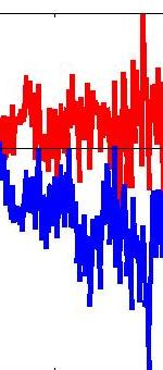
The right-hand panel shows the response of the linear filter, which is the inner product of the filter and the stimulus at every moment in time.
The red curve shows the response when the stimulus moves rightward; the blue curve shows the response when the stimulus moves leftward.
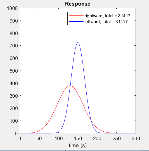
Here is the response as a function of time for both directions of motion. Notice that although the response to the leftward stimulus peaks at a much higher value, the total response is the same for both directions of motion. I had never realised this was the case until Damon pointed it out to me and found it hard to believe at first — although as the video makes clear, it’s just because in both cases the stimulus is sweeping out the same volume under the filter.
So can you describe this linear filter as direction-selective? It certainly gives a different response to the same stimulus moving rightward vs leftward, so I’d argue to that extent you can describe it as such. But since the total response is the same for both directions, it’s hard to argue it has a preferred direction. And it’s certainly true that to use it in any meaningful way, you’d want to apply a nonlinearity, whether squaring or a threshold or whatever. For example, if you wanted to use this “leftward filter” to drive a robot to turn its head to follow a leftward moving object, you’d be in trouble if you just turned the head leftward by an angle corresponding to the output of this filter. Sure the robot would turn its head left by so many degrees as an object passed left in front of it, but it would also turn its head left by the exact same angle if an object passed rightward! So in that sense, this filter is not direction-selective, and a nonlinearity is required to make it so.
Many thanks Damon and Jacob for taking the time to explain this to me!
The (slightly crummy) Matlab code I wrote to generate this video is below:
|
function JDirTest % This makes the tilted RF % Now run a nice simulation subplot(1,3,1) time = [0:300]; set(gca,’ydir’,’norm’) % Do inner product of current stimulus with filter: end end % do other direction % Stimulus is a Dirac delta function, x = vt + x0 end A Novel Form of Stereo Vision in the Praying MantisOur latest paper on mantis stereopsis has just come out in Current Biology. Briefly, we find that mantis stereopsis operates very differently from humans’: it is based on temporal change, and does not require the images to be correlated. We made a video abstract to explain the paper’s key findings and significance: Featured in National Geographic documentaryNational Geographic featured our work on mantis 3D vision in their recent documentary “Explorer: Eyes Wide Open”. Here’s a clip: Demo videos from our mantis 3D glasses paperWe uploaded 6 nice demo videos as Supplementary Material for our Scientific Reports paper. Unfortunately the links are currently broken (I have emailed) and in any case they are provided in a slightly clunky way where you have to download them. So I thought I would do a blog post explaining the videos here. Here is a video of a mantis shown a 2D “bug” stimulus (zero disparity). A black disk spirals in towards the centre of the screen. Because the disk is black, it is visible as a dark disk in both eyes, i.e. it’s an ordinary 2D stimulus. The mantis therefore sees it, correctly, in the screen plane, 10cm in front of the insect. The mantis knows its fore-arms can’t reach that far, so it doesn’t bother to strike. Loading Video Player….
Next, here’s a video of a mantis shown the same bug stimulus in 3D. Now the disk is shown in blue for the left eye and green for the right (bearing in mind that the mantis is upside down). Because the mantis’s left eye is covered by a green filter, the green disk is invisible to it – it’s just bright on a bright background, i.e. effectively not there, whereas the blue disk appears dark on a bright background. Loading Video Player….
Here’s a slo-mo version recorded with our high-speed camera. Unfortunately the quality has taken a big hit, but at least you get to see the details of the strike… Loading Video Player….
Sceptical minds (the best kind) might wonder if this is the correct explanation. What if the filters don’t work properly and there’s lots of crosstalk? Then, the mantis is seeing a single dark disk in our “2D” condition and two dimmer disks in our “3D” condition. Maybe the two disks are the reason it strikes, nothing to do with the 3D. Or maybe there’s some other artefact. As a control, we swapped the green and blue disks over, effectively swapping the left and right eye’s images. Now the lines of sight don’t intersect at all, i.e. this image is not consistent with a single object anywhere in space. Sure enough, the mantis doesn’t strike. Obviously, in different insects we put the blue/green glasses on different eyes, so we could be sure the difference really was due to the binocular geometry, not the colours or similar confounds. Loading Video Player….
Here’s the figure from our paper which illustrates this geometry and also shows the results: Fire and Light Yule Festival – with added science
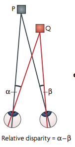
Stacey, Kathleen and I talked about how we see and perceive the world through light, with the help of some visual illusions and our ASTEROID 3D vision test. It was a great event and I’d like to do it again next year. Definitions of relative disparityI thought it might be useful to point out a property of relative disparity. One way is as Andrew Parker does in his 2007 review: Relative disparity = (alpha-beta) in the diagram below.
If P is not the fixation point, (alpha-beta) is not the absolute disparity of Q, but it is still the relative disparity between the points P and Q.
Parker (2007) says relative disparity = (alpha-beta). Read et al (2010) says relative disparity = (y-x). But look at the triangles. 180^o = x + z + alpha = y + z + beta. Thus, (alpha-beta) =(y-x) and the two definitions are identical.
COSYNE 2014Over in Salt Lake City at the moment for the Computational and Systems Neuroscience meeting. I always enjoy this meeting a lot and find it very stimulating. Looking forward to hearing some good talks over the next few days. Of nature and nurtureI’m no geneticist, but I was interested to see the recent comments on the heritability of academic performance. I thought it demonstrated the sorry lack of understanding of these things in the media and general public (including me), and I was disappointed in the quality of the debate. A government advisor, Dominic Cummings, wrote a report in the course of which he stated that “70% of cognitive capacity is genetic, beside which the quality of teaching pales into insignificance”. This got a lot of comment, e.e.g from Polly Toynbee in the Guardian. Toynbee does make clear that she doesn’t understand genetics, and seeks advice from genetics Prof Steve Jones. I eagerly heard a discussion of this on the BBC Radio 4 programme “Inside Science” between Profs Jones and Plomin, hoping they would give a clear explanation of what exactly heritability is which would help people like me. For example, Toynbee says at one point, “Wealth is considerably more heritable than genes”. This is obvious true in an everyday interpretation of the word – you can will your millions to your children, but you can’t guarantee they’ll inherit your striking red hair. But in the scientific definition of the word, nothing is more heritable than genes. I felt this demonstrated the confusion, and this is where we really needed a nice BBC science programme to go into these issues. Despite the august guests, I felt they didn’t really rise to the occasion. I’m no expert, but I find it helpful to realise that when we talk about heritability, we’re not talking about a fixed quantity, like the mass of the electron. It depends on the context. It may be 70% in Britain now, but it might have been 20% in the past and 90% in Finland. If you just consider one school where the kids come from similar backgrounds, the heritability may be close to 100% – there are bright kids and dimmer kids even within the same family, and it’s just how they are. But if you look between schools, comparing privileged vs deprived kids, you might find the variation between kids in each group is swamped by the large difference between the groups, indicating almost no heritability and an overwhelming effect of the environment. The closest the discussion got to this was a throw-away comment by Steve Jones: “If everyone stopped smoking, lung cancer would be a genetic disease”. I thought this was an important point which should have been pursued: if we could arrange things so that every child could get the best possible education to enable them to achieve their potential, academic performance would be 100% genetic. Finally,as far as I remember, no one stated that heritability has nothing to say about the importance of teaching quality, class size, resources and so on. If we find academic performance is 100% genetic, that indicates variation in these factors is not affecting results: children are receiving the same opportunities. But they may not be receiving the best opportunities. As I said above, I’m not a geneticist, so I’d welcome any correction if I’ve got the wrong end of the stick anywhere in the above… Mantis migrationThanks everyone who came along to help Lisa and me move our mantids across to their new home in the dedicated insect facility down the road. Especially Nick and Mike, who probably didn’t imagine when they came to the UK to do a MSc in Computer Games Engineering that this would involve transporting predatory insects! Although Nick — how about doing us a giant mantis in stereoanamorphic perspective? How scary would that be? Psychtoolbox MakeTextureI was just having a problem with MakeTexture in Psychtoolbox. I like to use “— In psychtoolbox@yahoogroups.com, “IanA” So I just needed to do |